cabelling

Abstract R code is provided in aide of laboratory demonstration of
cabelling.

1. Introduction

Setting up a cabelling experiment requires creating two watermasses of equal density, and if only S and T can be measured, that means calculating densities. Using a TS diagram and graphical interpolation is one approach to that task, but another is to use R to do the calculation.

2. Methods

The code given below will do the calculation for specified Sa, Ta and Sb, where the second letter indicates the watermass. The code uses uniroot() to find the temperature Tb that yields equal densities for watermasses “a” and “b”.

# Alter next three lines as desired; a and b are watermasses.
Sa <- 30
Ta <- 10
Sb <- 40
library(oce)
# Should not need to edit below this line
rho0 <- swRho(Sa, Ta, 0)
Tb <- uniroot(function(T) rho0-swRho(Sb,T,0), lower=0, upper=100)$root
Sc <- (Sa + Sb) /2
Tc <- (Ta + Tb) /2
## density change, and equiv temp change
drho <- swRho(Sc, Tc, 0) - rho0
dT <- drho / rho0 / swAlpha(Sc, Tc, 0)
if (!interactive()) png("cabelling.png", width=7, height=7,
                        unit="in", res=200, pointsize=12)
plotTS(as.ctd(c(Sa, Sb, Sc), c(Ta, Tb, Tc), 0), pch=20, cex=2)
drawIsopycnals(levels=rho0, col="red", cex=0)
segments(Sa, Ta, Sb, Tb, col="blue")
text(Sb, Tb, "b", pos=4)
text(Sa, Ta, "a", pos=4)
text(Sc, Tc, "c", pos=4)
legend("topleft",
       legend=sprintf("Sa=%.1f, Ta=%.1f, Sb=%.1f  ->  Tb=%.1f, drho=%.2f, dT=%.2f",
                      Sa, Ta, Sb, Tb, drho, dT),
       bg="white")
if (!interactive()) dev.off()

If run non-interactively, the code will produce a PNG file like that given below.

3. Results

The legend summarizes the results, indicating also the density change and the temperature change that would be equivalent to that density change (at the midpoint, “c”).

TS diagram for the setup of a cabelling experiment.

4. Conclusions

If the design goal is that the density mismatch between watermasses “a” and “b” should be, say, 10 percent of the density difference of the mixture watermass (“c”), then in the illustrated case the temperature would have to be controlled to within a quarter of a degree Celcius — a task that is challenging enough to argue against this as an informal classroom demonstration.

Exercises.

1. Alter the R code to calculate Sb in terms of Tb.
2. Consider (calculate or measure) the convection associated with sidewall heat conduction.

Pisa 2012 scores

The Guardian Newspaper has an interesting article about the Pisa (Program for International Student Assessment) scores for 2012, and it includes data. Since I was interested to see how my own region scored, I downloaded the data into a file called PISA-summary-2012.csv and created a plot summarizing scores in all the sampled regions, with Canada highlighted.

Summary graph, ranked in three categories

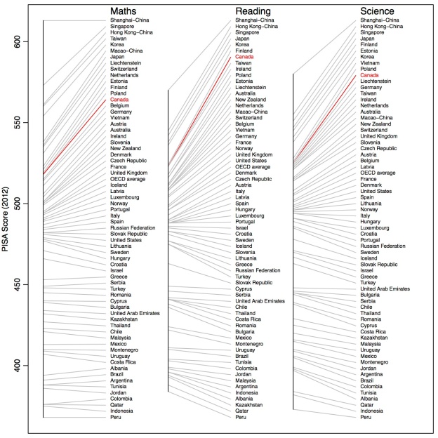
Summary of Pisa 2012 scores, broken down into category.

R code that creates the graph

The header length is unlikely to be the same in other years, nor the column names, so this code is brittle across similar datasets, but the necessary modifications for similar data should be obvious to anyone with passing familiarity with R.

regionHighlight <- "Canada"
d <- read.csv('PISA-summary-2012.csv', skip=16, header=FALSE,
              col.names=c("rank","region",
                          "math","mathLow","mathHigh","mathChange",
                          "reading",'readingChange',
                          'science','scienceChange'))
n <- length(d$math)
par(mar=c(0.5, 3, 0.5, 0.5), mgp=c(2, 0.7, 0))
range <- range(c(d$math, d$reading, d$science))
plot(c(0, 6), range,
     type='n', xlab="", axes=FALSE,
     ylab="PISA Score (2012)")
axis(2)
box()
dy <- diff(par('usr')[3:4]) / 50 # vertical offset

x0 <- 0
dx <- 1
cex <- 0.65

## Math
o <- order(d$math, decreasing=TRUE)
y <- approx(1:n, seq(range[2],range[1],length.out=n), 1:n)$y
segments(rep(x0, n), d$math[o], rep(x0+dx, n), y, 
     col=ifelse(d$region[o]==regionHighlight, "red", "gray"))
lines(rep(x0, 2), range(d$math))
text(rep(x0+dx, n), y, d$region[o], pos=4, cex=cex,
     col=ifelse(d$region[o]==regionHighlight, "red", "black"))
text(x0+dx, range[2]+dy, "Maths", pos=4, cex=1.2)

## Reading
x0 <- x0 + 2 * dx 
o <- order(d$reading, decreasing=TRUE)
segments(rep(x0, n), d$reading[o], rep(x0+dx, n), y, 
     col=ifelse(d$region[o]==regionHighlight, "red", "gray"))
lines(rep(x0, 2), range(d$reading))
text(rep(x0+dx, n), y, d$region[o], pos=4, cex=cex,
     col=ifelse(d$region[o]==regionHighlight, "red", "black"))
text(x0+dx, range[2]+dy, "Reading", pos=4, cex=1.2)

## Science 
x0 <- x0 + 2 * dx 
o <- order(d$science, decreasing=TRUE)
segments(rep(x0, n), d$science[o], rep(x0+dx, n), y, 
     col=ifelse(d$region[o]==regionHighlight, "red", "gray"))
lines(rep(x0, 2), range(d$science))
text(rep(x0+dx, n), y, d$region[o], pos=4, cex=cex,
     col=ifelse(d$region[o]==regionHighlight, "red", "black"))
text(x0+dx, range[2]+dy, "Science", pos=4, cex=1.2)

Contents of the PISA-summary-2012.csv data file

,,"Mean score
in PISA 2012, MATHS","Share
of low achievers
in mathematics
(Below Level 2)","Share
of top performers
in mathematics
(Level 5 or 6)","Annualised
change
in score points"," Mean score
in PISA 2012, READING","Annualised
change
in score points","Mean score
in PISA 2012, SCIENCE","Annualised
change
in score points"
1,Shanghai-China,613,3.8,55.4,4.2,570,4.6,580,1.8
3,Hong Kong-China,561,8.5,33.7,1.3,545,2.3,555,2.1
2,Singapore,573,8.3,40,3.8,542,5.4,551,3.3
7,Japan,536,11.1,23.7,0.4,538,1.5,547,2.6
12,Finland,519,12.3,15.3,-2.8,524,-1.7,545,-3
11,Estonia,521,10.5,14.6,0.9,516,2.4,541,1.5
5,Korea,554,9.1,30.9,1.1,536,0.9,538,2.6
17,Vietnam,511,14.2,13.3,m,508,m,528,m
14,Poland,518,14.4,16.7,2.6,518,2.8,526,4.6
13,Canada,518,13.8,16.4,-1.4,523,-0.9,525,-1.5
8,Liechtenstein,535,14.1,24.8,0.3,516,1.3,525,0.4
16,Germany,514,17.7,17.5,1.4,508,1.8,524,1.4
4,Taiwan,560,12.8,37.2,1.7,523,4.5,523,-1.5
20,Ireland,501,16.9,10.7,-0.6,523,-0.9,522,2.3
10,Netherlands,523,14.8,19.3,-1.6,511,-0.1,522,-0.5
19,Australia,504,19.7,14.8,-2.2,512,-1.4,521,-0.9
6,Macao-China,538,10.8,24.3,1,509,0.8,521,1.6
23,New Zealand,500,22.6,15,-2.5,512,-1.1,516,-2.5
9,Switzerland,531,12.4,21.4,0.6,509,1,515,0.6
26,United Kingdom,494,21.8,11.8,-0.3,499,0.7,514,-0.1
21,Slovenia,501,20.1,13.7,-0.6,481,-2.2,514,-0.8
24,Czech Republic,499,21,12.9,-2.5,493,,508,-1
18,Austria,506,18.7,14.3,0,490,-0.2,506,-0.8
15,Belgium,515,18.9,19.4,-1.6,509,0.1,505,-0.8
28,Latvia,491,19.9,8,0.5,489,1.9,502,2
-,OECD average,494,23.1,12.6,-0.3,496,0.3,501,0.5
25,France,495,22.4,12.9,-1.5,505,0,499,0.6
22,Denmark,500,16.8,10,-1.8,496,0.1,498,0.4
36,United States,481,25.8,8.8,0.3,498,-0.3,497,1.4
33,Spain,484,23.6,8,0.1,488,-0.3,496,1.3
37,Lithuania,479,26,8.1,-1.4,477,1.1,496,1.3
30,Norway,489,22.3,9.4,-0.3,504,0.1,495,1.3
32,Italy,485,24.7,9.9,2.7,490,0.5,494,3
39,Hungary,477,28.1,9.3,-1.3,488,1,494,-1.6
29,Luxembourg,490,24.3,11.2,-0.3,488,0.7,491,0.9
40,Croatia,471,29.9,7,0.6,485,1.2,491,-0.3
31,Portugal,487,24.9,10.6,2.8,488,1.6,489,2.5
34,Russian Federation,482,24,7.8,1.1,475,1.1,486,1
38,Sweden,478,27.1,8,-3.3,483,-2.8,485,-3.1
27,Iceland,493,21.5,11.2,-2.2,483,-1.3,478,-2
35,Slovak Republic,482,27.5,11,-1.4,463,-0.1,471,-2.7
41,Israel,466,33.5,9.4,4.2,486,3.7,470,2.8
42,Greece,453,35.7,3.9,1.1,477,0.5,467,-1.1
44,Turkey,448,42,5.9,3.2,475,4.1,463,6.4
48,United Arab Emirates,434,46.3,3.5,m,442,m,448,m
47,Bulgaria,439,43.8,4.1,4.2,436,0.4,446,2
43,Serbia,449,38.9,4.6,2.2,446,7.6,445,1.5
51,Chile,423,51.5,1.6,1.9,441,3.1,445,1.1
50,Thailand,427,49.7,2.6,1,441,1.1,444,3.9
45,Romania,445,40.8,3.2,4.9,438,1.1,439,3.4
46,Cyprus,440,42,3.7,m,449,m,438,m
56,Costa Rica,407,59.9,0.6,-1.2,441,-1,429,-0.6
49,Kazakhstan,432,45.2,0.9,9,393,0.8,425,8.1
52,Malaysia,421,51.8,1.3,8.1,398,-7.8,420,-1.4
55,Uruguay,409,55.8,1.4,-1.4,411,-1.8,416,-2.1
53,Mexico,413,54.7,0.6,3.1,424,1.1,415,0.9
54,Montenegro,410,56.6,1,1.7,422,5,410,-0.3
61,Jordan,386,68.6,0.6,0.2,399,-0.3,409,-2.1
59,Argentina,388,66.5,0.3,1.2,396,-1.6,406,2.4
58,Brazil,391,67.1,0.8,4.1,410,1.2,405,2.3
62,Colombia,376,73.8,0.3,1.1,403,3,399,1.8
60,Tunisia,388,67.7,0.8,3.1,404,3.8,398,2.2
57,Albania,394,60.7,0.8,5.6,394,4.1,397,2.2
63,Qatar,376,69.6,2,9.2,388,12,384,5.4
64,Indonesia,375,75.7,0.3,0.7,396,2.3,382,-1.9
65,Peru,368,74.6,0.6,1,384,5.2,373,1.3